What Changed
On March 8, the 2026 Hormuz disruption was 8 days old. The mixture model placed 55% probability on a rapid de-escalation branch, producing a median forecast of just 13 days for the mixture-only model and 88 days for the full two-stage model (with reopening lag).
It is now March 19, 2026 — day 19 of the disruption. The strait has not reopened. No political off-ramp has materialized. The key question: how does the forecast change given what we've observed?
The Bayesian Update
Recall that the mixture model is not memoryless. Each component (exponential) is memoryless individually, but the mixture as a whole is not. As time passes without resolution, the posterior weight on the de-escalation branch declines — the model "learns" that the quick-exit scenario has become less plausible.
Formally, the posterior weight on the de-escalation branch after observing survival to day t is:
where S(t) is the mixture survival function evaluated at t. The de-escalation hazard (λD ≈ 0.179 / day) is 178× faster than the baseline Hormuz hazard (λH ≈ 0.001 / day), so the de-escalation branch's contribution to S(t) decays exponentially fast.
Posterior Weight at Day 19
The de-escalation weight has collapsed from 55% to under 4%. In plain terms: the model's "quick exit" scenario has been almost entirely consumed by the passage of 19 days without any sign of political reversal. The forecast now looks nearly identical to the long-duration baseline Hormuz profile.
Weight Decay Over Time
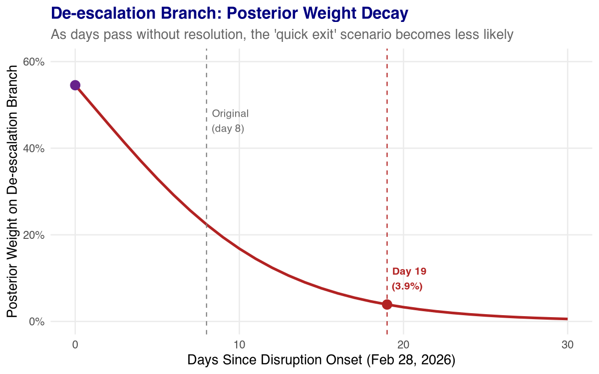
Figure 1. Posterior weight on the de-escalation branch over the first 30 days. By day 19, the weight has decayed from 54.5% to 3.9%. The trajectory is governed by the ratio of de-escalation to baseline hazard rates (178×).
This is the non-memoryless property in action. Each passing day without resolution makes the de-escalation branch exponentially less probable. By day 30, the weight would fall below 1%. The mixture model self-corrects as data arrives.
Updated Forecasts
Updated Mixture Only (Stage 1)
With the posterior weights updated to pD = 3.9% and pH = 96.1%, the conditional distribution of remaining duration from today is:
Updated Mixture Forecast: Remaining Duration
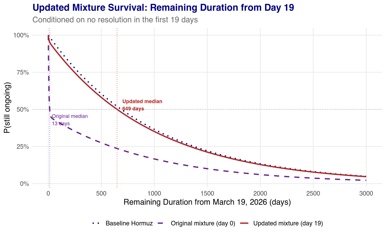
Figure 2. Updated mixture survival (solid red) vs. original mixture (dashed purple) vs. baseline Hormuz (dotted blue). The updated mixture has converged toward the baseline.
Comparison: Mixture Only
| Quantity | Original (day 8) | Updated (day 19) | Change |
|---|---|---|---|
| De-escalation weight | 54.5% | 3.9% | −50.6 pp |
| Mean remaining | 454 days | 951 days | +497 days |
| Median remaining | 13 days | 647 days | +634 days |
| 90th percentile | 1,504 days | 2,238 days | +734 days |
The median has shifted from 13 days to 647 days — a 50× increase. This is the single most informative number in the update: the model's best single point estimate for remaining duration has moved from "about two weeks" to "about 1.8 years."
Updated Two-Stage Forecast (Mixture + Reopening Lag)
Adding the reopening-lag layer (unchanged from the original article: 7–14 days at 30%, 21–45 days at 50%, 60–120 days at 20%):
Updated Full Forecast: Time to Meaningful Transit
Probability of Reopening Within Key Horizons
| Question | Original (day 8) | Updated (day 19) |
|---|---|---|
| Meaningful transit within 30 days? | ~21% | ~2% |
| Meaningful transit within 90 days? | ~51% | ~9% |
| Meaningful transit within 180 days? | — | ~17% |
| Meaningful transit within 1 year? | — | ~31% |
| Still materially impaired after 60 days? | ~56% | ~94% |
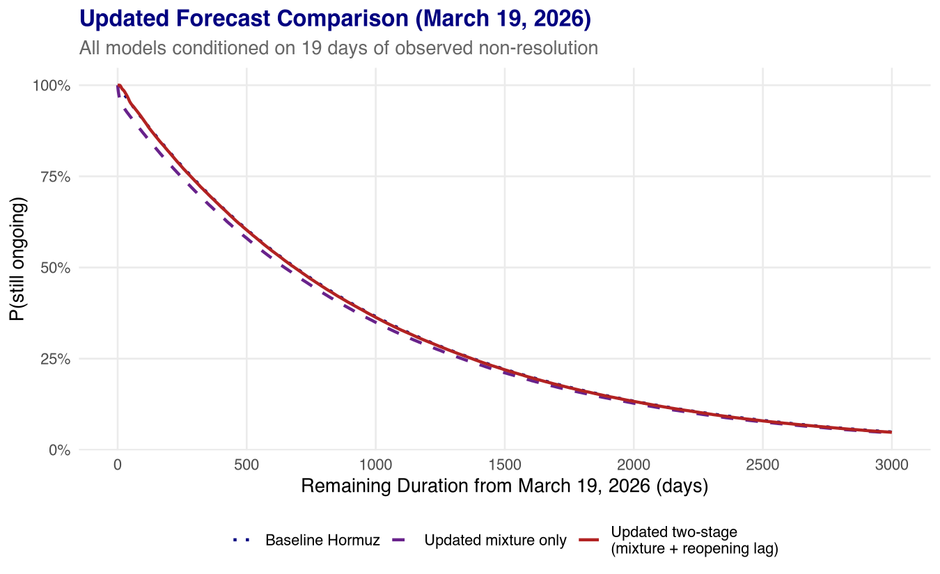
Figure 3. Updated forecast comparison: solid red = full two-stage model (mixture + reopening lag), dashed purple = mixture only, dotted blue = baseline Hormuz only. All conditioned on T > 19 days.
Interpretation
The update tells a clear story: the window for a rapid de-escalation resolution has essentially closed.
On March 8, the model placed meaningful probability (~55%) on a scenario where the disruption resolves within days or weeks, calibrated from the observed pattern of rapid tariff-decision reversals. Eleven days later, with no sign of resolution, the model has updated that probability down to under 4%.
The practical implication: the forecast now closely resembles the baseline Hormuz exponential model, which is calibrated from five historical disruption episodes ranging from 138 days (2019) to 2,652 days (Tanker War). The median remaining duration is approximately 1.8 years, the mean is approximately 2.7 years, and there is only about a 31% probability of meaningful shipping transit resuming within one year.
This is exactly how the model was designed to work:
- The mixture model converts passage of time into Bayesian evidence against the quick-exit scenario.
- The rapid decay of the de-escalation weight (178× hazard ratio) means the model updates decisively — it does not linger in ambiguity.
- After roughly 3–4 weeks, the de-escalation branch becomes negligible and the forecast converges to the historical base rate.
Sensitivity: Influence of Individual Episodes
The baseline Hormuz model is fitted to just five episodes. A natural concern: does any single episode dominate the estimate? To answer this, I refit the exponential model five times, each time dropping one episode and computing the MLE from the remaining four. This leave-one-out (LOO) analysis makes each episode's influence transparent.
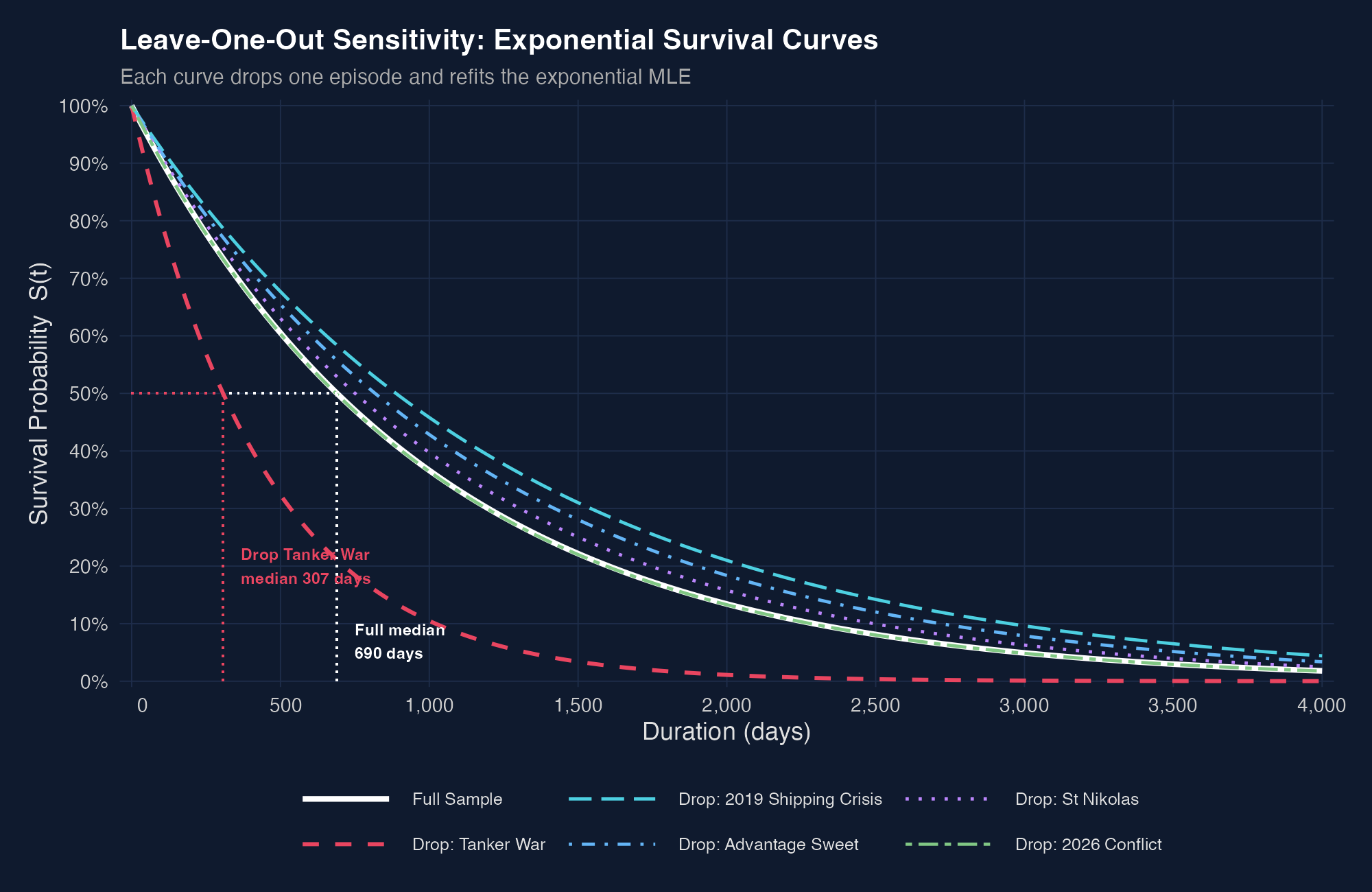
Figure 4. Leave-one-out exponential survival curves. Each colored curve drops one episode and refits the MLE. The full-sample curve is shown in white. The "Drop Tanker War" curve (red, dashed) is visually separated — removing the Tanker War roughly doubles the hazard rate.
LOO Summary
| Dropped Episode | Events (d) | Exposure (Σt) | λ̂ | Mean | Median |
|---|---|---|---|---|---|
| Tanker War | 3 | 1,330 | 0.00226 | 443 days | 307 days |
| 2019 Shipping Crisis | 3 | 3,844 | 0.00078 | 1,281 days | 888 days |
| Advantage Sweet | 3 | 3,541 | 0.00085 | 1,180 days | 818 days |
| St Nikolas | 3 | 3,250 | 0.00092 | 1,083 days | 751 days |
| 2026 Conflict | 4 | 3,963 | 0.00101 | 991 days | 687 days |
| Full Sample | 4 | 3,982 | 0.00100 | 995 days | 690 days |
What to make of this:
- The Tanker War contributes 67% of total exposure time (2,652 of 3,982 days). Dropping it roughly doubles the hazard rate and halves the median forecast — from 690 days to 307 days.
- No other single episode moves the estimate by more than ~30%. The model is not uniformly sensitive to every observation — it is specifically sensitive to the Tanker War.
- This does not mean the Tanker War should be excluded. It was a real, multi-year interstate conflict that disrupted Hormuz traffic. But readers should understand that the forecast's long right tail is substantially driven by one historical episode that may or may not be representative of the current geopolitical context.
- A reasonable interpretation: the range between the "drop Tanker War" median (~10 months) and the full-sample median (~23 months) brackets the plausible baseline forecast, depending on whether one views the current conflict as comparable to a full interstate war or to the shorter diplomatic/detention episodes.
How Long? Prediction Intervals
The point estimates above (median ~690 days, mean ~995 days) treat the hazard rate λ̂ as known. But with only 4 observed events, uncertainty in λ itself is substantial. A statistically principled forecast should propagate this parameter uncertainty into the prediction.
The Bayesian posterior predictive does exactly this. Under a non-informative prior, the posterior for λ is Gamma(4, 3982), and the predictive distribution for remaining duration follows a Lomax distribution with closed-form quantiles. This distribution is heavier-tailed than the point-estimate exponential — reflecting the real possibility that the true hazard rate is lower (i.e., disruptions last longer) than our best estimate.
Posterior Predictive: Remaining Duration from March 19, 2026
Prediction Intervals
| Interval | Lower Bound | Upper Bound | Interpretation |
|---|---|---|---|
| 50% PI |
297 days Jan 2027 |
1,649 days Sep 2030 |
Even odds the disruption lasts between ~10 months and ~4.5 years |
| 80% PI |
106 days Jul 2026 |
3,099 days Sep 2034 |
Likely range: ~3.5 months to ~8.5 years |
| 95% PI |
25 days Apr 2026 |
6,032 days Sep 2042 |
Near-certainty bounds: ~1 month to ~16.5 years |
Reading the table:
The 50% prediction interval says there is a 50% probability that the
remaining disruption duration falls between ~10 months and ~4.5 years. The interval is wide
because the underlying data is sparse — 4 resolved episodes spanning 138 to 2,652 days — and
the Bayesian predictive honestly reflects that uncertainty.
The median of ~2.1 years (April 2028) is the single best point forecast:
it is equally likely the disruption ends sooner or later than this date.
The mean of ~3.6 years is substantially higher because the distribution has a
long right tail — there is meaningful probability of a very long disruption, consistent with
the Tanker War precedent.
These intervals describe the political/military disruption duration. The
reopening-lag model (unchanged from the original article) adds approximately 38 days on average
for the operational process of restoring commercial traffic after a political resolution.
Prior-Informed Scenario: What Does Substantive Analysis Say?
The prediction intervals above are derived purely from historical base rates. But a Jaynesian critique applies: with only 4 observed events, the model is mostly reporting back its assumptions. The most honest analysis acknowledges this and asks: what does substantive knowledge about the current conflict actually imply?
The current conflict is structurally unprecedented among the five historical episodes:
- The US is a primary combatant, not a neutral escort (as in the Tanker War). Trump's demonstrated preference for short, decisive operations (cf. the Venezuela incursion) suggests a compressed timeline — but Iran's capacity to fight back creates genuine uncertainty.
- The scope is existential — regime decapitation, 7,000+ strikes, the deaths of Khamenei and Larijani. This isn't a shipping harassment campaign.
- Regional contagion is unprecedented — strikes on Ras Laffan, the Strait reduced to a dead zone (97% traffic reduction vs. 2% in the 1980s).
These factors suggest the disruption may resolve faster than the historical base rate implies (because the military campaign is so intense) or could spiral into a prolonged regional crisis (because the stakes are existential). To formalize this tension, I calibrate a prior distribution from stated beliefs about the current conflict:
Elicited Prior Calibration:
- "I'd be surprised if this goes beyond 4 months" → P(remaining > 120 days) ≈ 15%
- "I'd be shocked if it goes beyond a year" → P(remaining > 365 days) ≈ 3%
- "I'd be shocked if it ends tomorrow" → P(remaining < 1 day) should be very small
- "I can't rule out 1,095 days or 4 hours" → fat tails in both directions
These constraints uniquely determine a LogNormal(μ = 3.42, σ = 1.32) distribution. The log-normal naturally accommodates the asymmetry: a sharp concentration in the 2–16 week range with a long right tail that doesn't rule out multi-year outcomes.
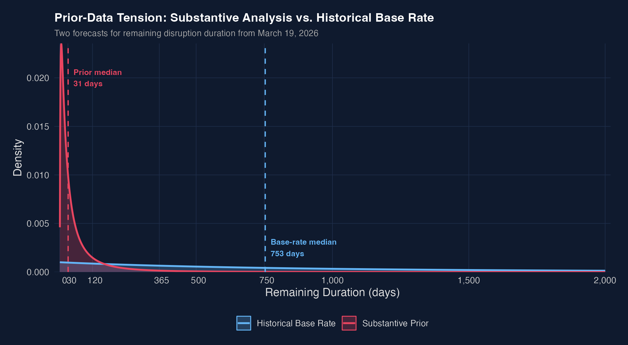
Figure 5. The substantive prior (red) concentrates mass in the first few months; the historical base rate (blue) assigns most probability to durations measured in years. The medians differ by a factor of 24×.
Comparison: Base Rate vs. Substantive Prior
| Quantity | Historical Base Rate | Substantive Prior |
|---|---|---|
| Median | 753 days (~2.1 yr) April 2028 |
31 days (~1 mo) April 2026 |
| Mean | 1,327 days (~3.6 yr) Nov 2029 |
73 days (~2.4 mo) May 2026 |
| 50% PI | 297 – 1,649 days | 13 – 75 days Apr – Jun 2026 |
| 80% PI | 106 – 3,099 days | 6 – 166 days Mar – Sep 2026 |
| 95% PI | 25 – 6,032 days | 2 – 405 days Mar 2026 – Apr 2027 |
The honest answer:
The historical base rate and the substantive analysis are in sharp disagreement — their medians differ by a factor of 24×. With only 4 historical events, the data cannot resolve this tension. The reader's forecast should depend on how much weight they assign to:
- Historical persistence ("Hormuz disruptions have lasted years before, and base rates are hard to beat") → base-rate model, median ~2 years
- Current tactical dynamics ("This is a qualitatively different conflict with a decapitation strategy and unprecedented firepower") → substantive prior, median ~1 month
Both positions are defensible. Reporting both — rather than collapsing to a single forecast — is the most informative thing this analysis can do.
Unchanged Assumptions
This update conditions the forecast on new data (19 days elapsed) but does not change any model parameters:
- The baseline Hormuz hazard (λH = 0.001007/day) remains as estimated from the five-episode dataset.
- The tariff-retreat calibration (λD = 0.1791/day, p₀ = 0.545) remains as of the March 8 cutoff.
- The reopening-lag distribution (three-scenario uniform mixture) remains unchanged.
The forecast changes entirely through the Bayesian posterior update — not through parameter re-estimation.
Conclusion
Nineteen days into the 2026 Strait of Hormuz disruption, the mixture model's Bayesian update has nearly exhausted the de-escalation scenario. The forecast has shifted from a bimodal profile (short or very long) to a unimodal, long-duration profile consistent with the historical base rate.
The updated full two-stage forecast (mixture + reopening lag) gives a median time to meaningful transit of approximately 685 days (~1.9 years), with only a ~2% probability of reopening within 30 days and a ~94% probability that traffic remains materially impaired after 60 days.
As with the original article, these are descriptive estimates based on small historical samples and cross-domain calibration — not structural forecasts. But the Bayesian update mechanism provides a principled way to incorporate the most important new information: the disruption is still ongoing.